Additive Mixtures Video

@daniele , excellent video. I really enjoyed it! It clearly highlights the issue of conflating “scene-referred” with scene colorimetry, an inference implied by ISO 22028 but not discussed in Kodak’s early development of these concepts. At Kodak, our scene-referred models often produced exposure values rather than CIE XYZ values, and I think the video is an excellent illustration of exactly why. In the context of this conversation, exposure values, or camera tristimulus values, are the result of integrating scene radiance with the capture medium’s spectral sensitivities. As your video suggests, the goal of an IDT in ACES is to map those varied exposure values from different capture media into a single space. You mentioned normalizing all cameras to a specific camera space, which is essentially the purpose behind defining the Reference Capture Input Device (RICD). The RICD just happens to have spectral sensitivities that are a linear combination of the color matching functions. We could have easily chosen a different set of spectral sensitivities for the RICD, but it may have been very difficult to communicate why they were chosen.

Your video brought up an interesting point I hadn’t considered deeply before: values outside the spectrum locus, when converting to ACES through an IDT, are not a flaw but actually a feature. This allows for the preservation of the original color ratios present in the camera exposure values. This makes obvious sense in retrospect, but you highlight the clear downside of using non-linear IDTs in your video. Using a linear transform to achieve this maintains the unique characteristics of each camera as they are mapped into a common space, while a non-linear transform would alter the original camera exposure ratios. If values lie outside the RICD space, the responsibility falls to those handling these values downstream to ensure they are appropriately mapped back in. The requirements for mapping may be different depending on the specific operations being performed. This is something we discussed in the early days of ACES, but your point that keeping those original R, G, B relationships intact could be crucial for some operations, is one that I think has been understated.

Very thought provoking video.

3 Likes

This seems problematic? The “energy” we are discussing is always in relation to the neurophysiological signals, and by forcing things to a Cartesian world view of infinite Grassmann additivity, the technique actually creates a problem that does not entirely exist in the closed domain, post FPGA quantal catch counts1.

I believe it would depend on the nature of the “non-linear” transform?

Are there implications in the formed pictorial depictions, then?

1 In the case of pictorial depictions, it is quite possible that the catch counts will have energy relationships that will be problematic in forming a picture. EG: A very narrow spectral filtration can yield egregiously low values that will manifest as uncanny energy regions in pictorial depictions.

I think this is exactly contradictory to @daniele point. He’s saying this has nothing to do with human color stimulus but the stimulus of the medium on which the image was captured. Perception/ psychology is a whole separate realem from this discussion.

Maybe but give a concrete example

What exactly do you mean by “formed pictorial depictions?” Are you still talking scene state? Is it not enough that the exposure values are dependent on the spectral sensitivities? Should we also consider cross talk? Digital camera code values have that.

Thank you @Alexander_Forsythe , glad you liked it.

I agree that “finally” once we have formed an image we need to correlate the signal to the human observer.
But my point is, to do that we need to preserve as much of the original information as possible. And colourimetry information is not the only type of information that counts. And it is unsharp.
I think you would agree.

That is an interesting point. The past shows two things:

  • uncareful “bending” of additive mixtures cause all sorts of problems
  • some image pipelines (like film) inherently bend additive mixtures and we do not seem to have a problem with that

I think we need some research in this area to get a framework which guides us on the way from scene to display(s).

I don’t want to make a religion out of additive mixtures. Clearly none linear transforms are successfully used in our industry. I am just saying, we should not put it at the very first step of the chain. And we should appreciate those modern cameras.

This is an interesting point, I would not even know how to phrase sharp objectives. But I think this could be an interesting realm for many thought experiment.

Not in the least?

For Grassmann additivity to even remotely hold in the extremely limited increment test state of extreme low articulation, it would imply there is a direct path between the “presented” energy and the neurophysiological signals?

We aren’t “seeing” object A “over” object B. We are forming and shaping that information cognitively, up and out of the neurophysiological signals.

It’s a picture of “motion blur”? How do we interpret that? Why do the @TooDee star demonstrations lead to a cognition that is not “over” the ground?

Aren’t those all probabilistic inferences based upon the stimuli fields presented in the pictorial depictions? It’s not “physics” of “a scene”. It could be a painting.

Don’t get me wrong, CAMs and UCSs and everything else that tries to sell their ridiculous model ideas are verifiably false without much effort to disprove their veracity. So I agree, they have no place in this discussion at all. We can probably blame Hunt for this rubbish, and he would have done well to listen to Land.

The thing we are looking at is a formed pictorial depiction? The energy fields present in the pictorial depiction are interpreted by our top down processing. The relationships between the gradient fields are what leads us to the inferences?

When we pooch the formed pictorial depiction, the probability that we infer the intended authorial depiction will increase or decrease based on the spatiotemporal gradient fields.

“Scene” is a myth under this lens? There is only the pictorial depiction which serves as the canonized material to be read and interpreted?

The exposure values don’t matter if the energy relationships within the picture’s gradient fields disrupt and violate the general idea? This is verifiable in all of the “Colour Appearance Models” and “Uniform Colour Spaces”.

I don’t believe this is correct? Electrical sensors can only ever report the quantal catch gains. There is no signal cross talk in the sense of chemical creative film, nor is there a density metric present which leads to an offset and normalization of the stimuli fields.

This is probably the most “essential” difference between chemical film and electrical sensors?

I agree that there seems to be an energy relationship buried in this. But I would again draw attention to three points that we continually “forget”:

  1. We are looking at a formed pictorial depiction of “blur” or “over” etc. We need to focus on the energy state of the formed picture because we can see how bogging up this energy clearly leads to cognitive fission errors, that have a lower probability of the fission taking place. “The star does not look ‘blurry’ and in front of the ground.” “Her hand does not look ‘in motion’ in the static picture.”
  2. We are failing to formally bolt down what the energy is. We know that the energy will be decomposed into an opponency signal chain that leads to portions of the energy being “negated” by way of inhibition.
  3. We already have some of this energy relation at the electrical quantal catch. Sharp, low or no integral filtration can disrupt the fields, which will become deeper problems in formed pictures. EG: “Clefts” from some of the earlier CCD sensors where the spectral characterizations had “gaps” between them. We can have a broken pictorial depiction if the sensor quantal catch is “too low”.

We would be wise to outline what “additivity” means? It is not something outside of us.

This! We would be incredibly wise to evaluate what the broad foundational thresholds are for the probability of a cognition of “over” or “under”?

To pictorial depictions? It’s not about a display any more than Impression, Sunrise is about “scene” to “display”; the articulations of the presented pictorial fields exist on a probabilistic curve of “that looks over that”, as a result of the formed fields.

image

May I ask what RICD is? I googled it, but not sure I understand what it means.

ACES terminology introduced in [61] defines a Reference Image Capture Device (RICD) as an ideal/virtual colorimetric camera whose sensor’s spectral sensitivities record scene luminance directly in the above color-space (i.e., linearity between scene relative exposure and CVs) [35]. RICD is defined void of system noise, with 0.5% camera flare off a perfect reflecting diffuser, whose reflected light from a standard D60 illumination source (i.e., a 100% reference-white) is scaled to CV (1.0, 1.0, 1.0), whereas the same recorder light off an 18% grey card maps to CV (0.18, 0.18, 0.18). The viewing environment is always considered observer-adaptive to D60, with 1600 cd/m2 minimum adapted luminance and 0% viewing flare.

Is it essentially Linear AP0 ACES 2065-1?
But the part about 0.5 camera flare makes me think it isn’t. If I get it right, ACES 2065-1 places 0.0 to 0.0.

The RICD is a theoretical camera that produces ACES 2065-1 values directly.

ACES 2065-1 is supposed to have a small amount of flare in it. It’s specified as having that flare so one doesn’t think they have to remove the flare from real world images to encode them as ACES 2065-1. It’s only a guideline as any deviation is considered creative intent.

I think there’s a slight mistake in the quote from Walter’s paper. Normally, you scale so that 18% in the scene ends up at 0.18, but because of the flare 100% scene white won’t come out at exactly 1.0.

1 Like

Thought I’d post this here since the other thread is knee deep in a Lovecraftian orgy of number fornication, with the hope of Yog-Sothoth being summoned.

There seems to be an assumption that “the colour” is in the pictorial depiction. I’d suggest this is not the case, and broadly patterns after a Grossbergian idea around “response normalization”1.

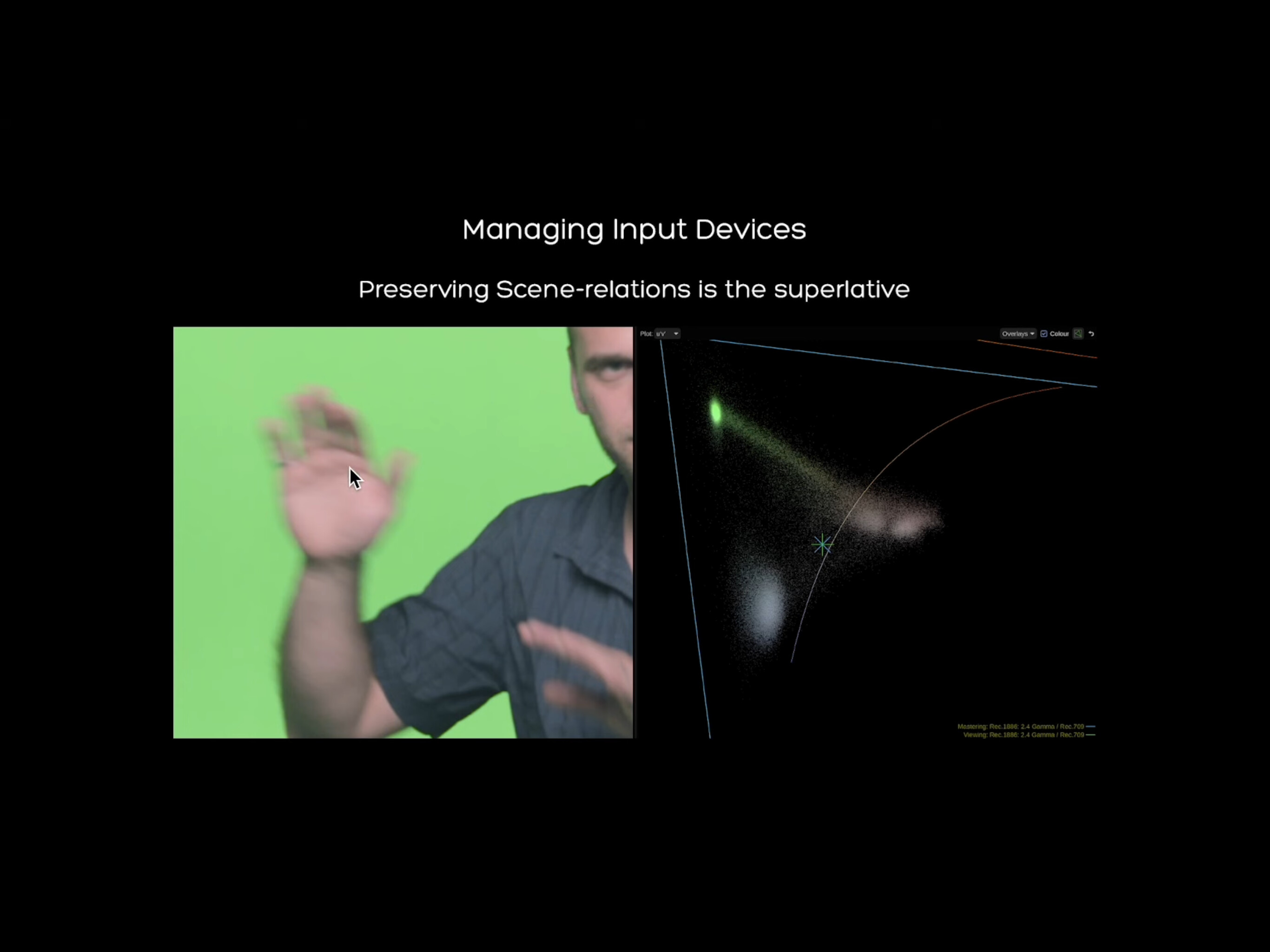
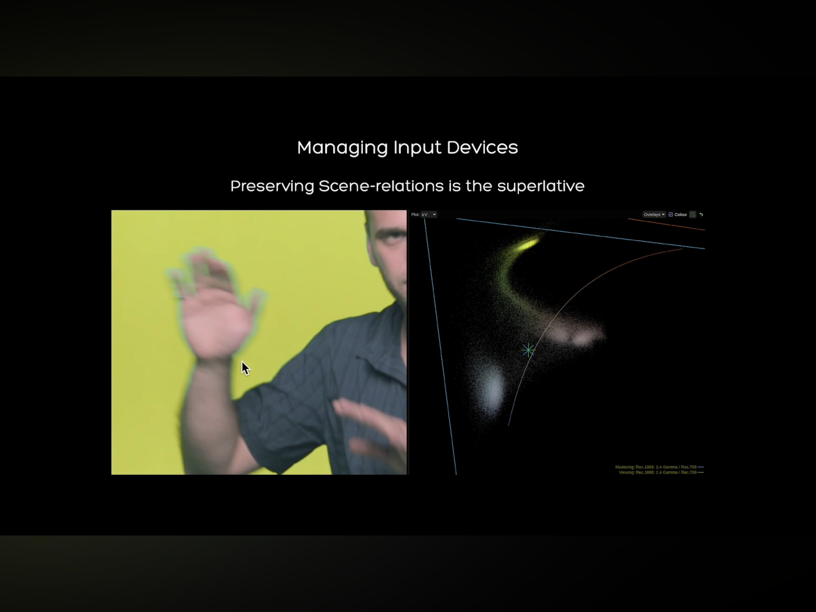
When we look at a pictorial depiction of “motion blur” I would suggest that we are fissioning the forms / entities into a decomposition based on probabilities of something “over” some other “form”. Daniele’s videos show some of this rather nicely, although @TooDee has been trying to draw attention to this for a long time, and sadly no one has been paying attention.

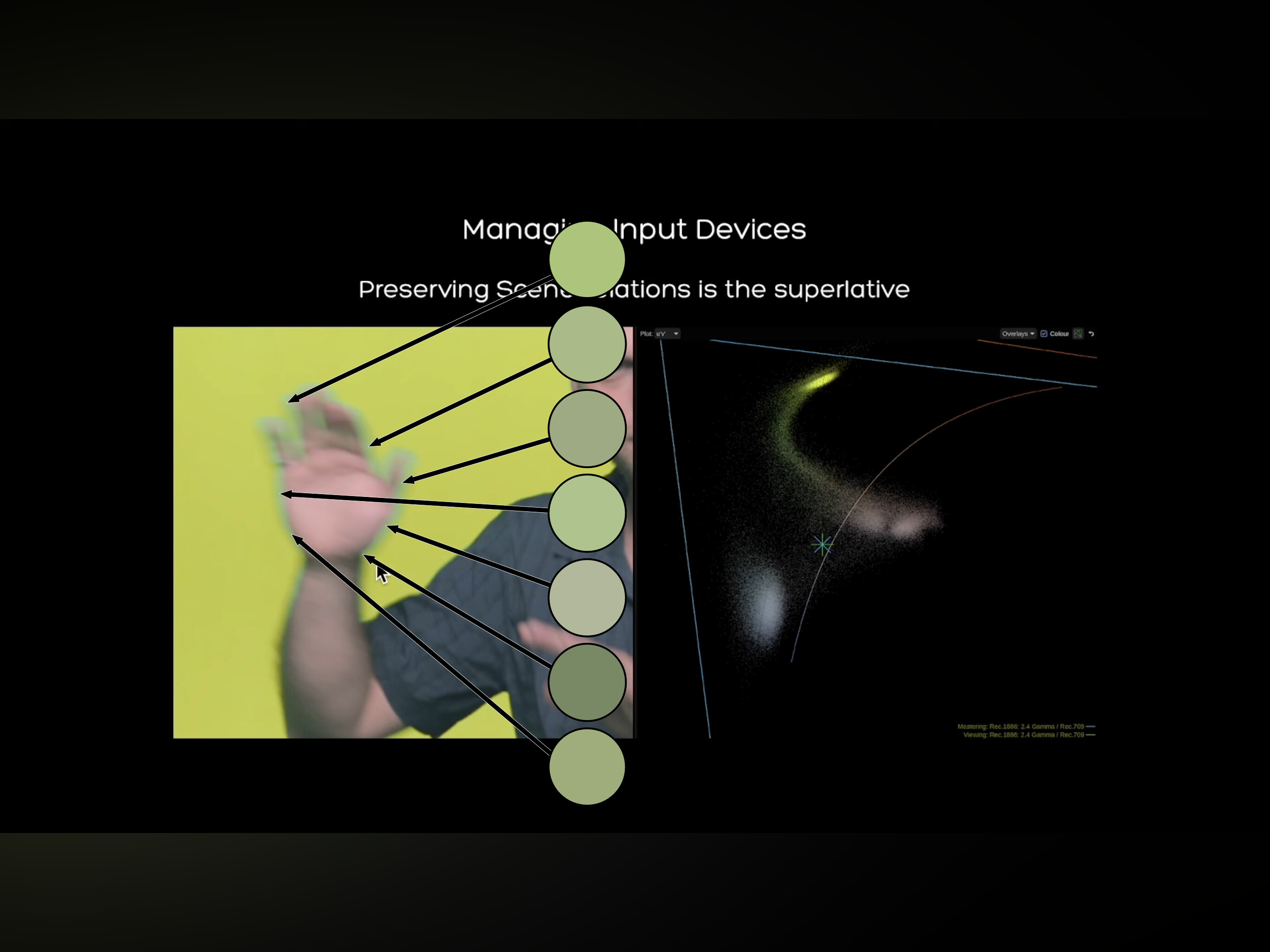
Here are the two demonstrations selects that I pulled from the video. Pay attention to the “hand” depiction, which can be challenging with the depiction of a “rugged Italian German” cropped at the right of the frame:

I believe it is important to wipe away all of our nonsense about “scene” and “display” for a moment and realize that what we are parsing are the pictorial fields presented to us right now.

We can clearly see that in one case the pictorial form leads to “hand of rugged Italian German on ground of ‘green’” and in the other “hand of rugged Italian German with a tremendous looking grape-like forehead on a ‘ground’ of ‘yellowish’, and a ‘ring’ around the ‘hand’.”

But these ideas are a tad deceptive, and I would suggest that we are engaging in the aforementioned response normalization by way of the neurophysiological signal energies.

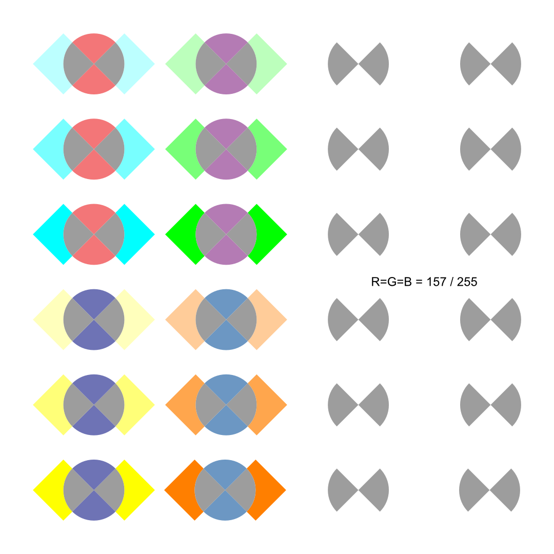
First up… Let’s see if the “colour” we think we are seeing is present within the stimuli:

I’ll go out on a limb and suggest that most would agree that the cognized computed colour that we think is “around” the “hand” is an unsatisfactory match to any singular stimuli sample. Feel free to reject this idea, and find a better sample.

So this leads to the question, if the colour we are cognitively computing by way of the fissioning mechanism / normalization, is not present in the stimuli, what specific facet of the gradient is leaning our probability computation to read the stimuli as “other”, and a “ring” around the hand?

The answer thankfully must be present in the stimuli presented in the pictorial depiction, without falling into Giorgianni-Kodak’s bunko rabbit hole of “scene” and “display”. We could say that there’s a rather tenuous link between the gradients present in the quantal catches, as Daniele has showcased, but in the end, what we are presented with in the pictorial depiction is all the evidence we likely need to diagnose the crime scene. And we know that a physicalist energy cannot account for this phenomena, as the computation is meatware based, from the neurophysiological signals. Somehow we are fissioning out the “cyan green” “ring” around the “hand” from the “yellow slime” “ground”, and the “pale pink-yellow” depiction of “hand”.

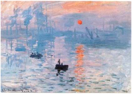
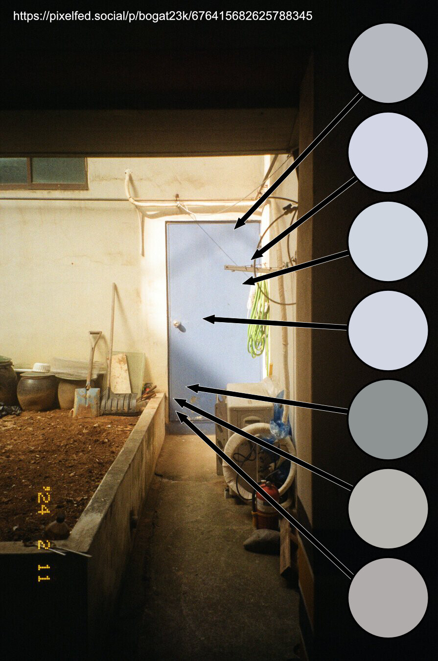
I’ve been sort of fascinated by this local response normalization by tracking how chemical film introduces the offset dimension2, where electrical sensors do not. Might be interesting to some folks. The picture a film scan from Pixel Fed’s Bogat23k:

The key point is that our computation of the “blueness” of the door is plausibly an unsatisfactory “match” to any given sample of stimuli. Somewhere in this cognitive fission mechanism we should be able to spot a pattern of local differential gradients.

If we loop back to the Daniele “hand” depiction, we can get a sense that at a given spatial viewing frustum3 the depiction of the “hand” is cutting across “three” differential gradient boundary “slope zeros”, and our meatware computation might be triggering on these as high probabilities of “boundary” as opposed to “same”.

1 This has a massive amount of research papers, but this one is useful for a broad summary of the idea of normalization around pools / fields of neurons. Carandini, Matteo, and David J. Heeger. “Normalization as a Canonical Neural Computation.” Nature Reviews Neuroscience 13, no. 1 (January 2012): 51–62. Normalization as a canonical neural computation | Nature Reviews Neuroscience.
2 I strongly believe that the totality of the cognitive fission response normalization can be mapped along gain to offset dimensions, and that the crucial difference between chemical creative film and crappy electronic sensor data rests in this dimensional projection. One integrates the offset, one can only integrate the gain, and leaves the formulation of the offset dimension to the pictorial formation algorithms. Which leads us to the Lovecraftian Orgies of Yog-Sothoth.
3 I would suggest that viewing frustum dimension must be crucially important here for we can “zoom out” to a point where we would suggest a low probability of “boundary”, and likewise “zoom in”. That is, the physical energy that lands on our log-polar density of cells is likely influencing the differential gradients of the On-Off / Off-On cells. Viewing frustum matters of course, for anyone who has sat in front of a 40 meter screen and experienced iPhone level camera shake probably would attest.

3 Likes

Hi Troy, crosstalk mentionned by @Alexander_Forsythe is most likely not referring to electronic crosstalk but spectral crosstalk caused by the RGB filters and sensor spectral sensitivity. In that context, the process is similar to film.

1 Like

A bit dated but the physics still hold

I agree that there’s a sort of “crosstalk” of terms here.

I’d be reluctant to label a spectral sensitivity overlap as “crosstalk”. Perhaps it’s another one of those words that is past its best before date.

I don’t believe that spectral sensitivity overlaps have much to do with the discussion point here, but I am open to being proven wrong if someone can make a case for it. In the end, the idea of an infinite Grassmann additivity is already accounting for the overlaps, and the resulting gained stimuli “magic” is happening at the neurophysiological level.

1 Like

Sorry, I confused crosstalk with what we called cross-coupling in film. @Alexander_Forsythe was indeed referring to electronic/optical/photonic crosstalk (his reply above).